Intro
Recall the following figure:
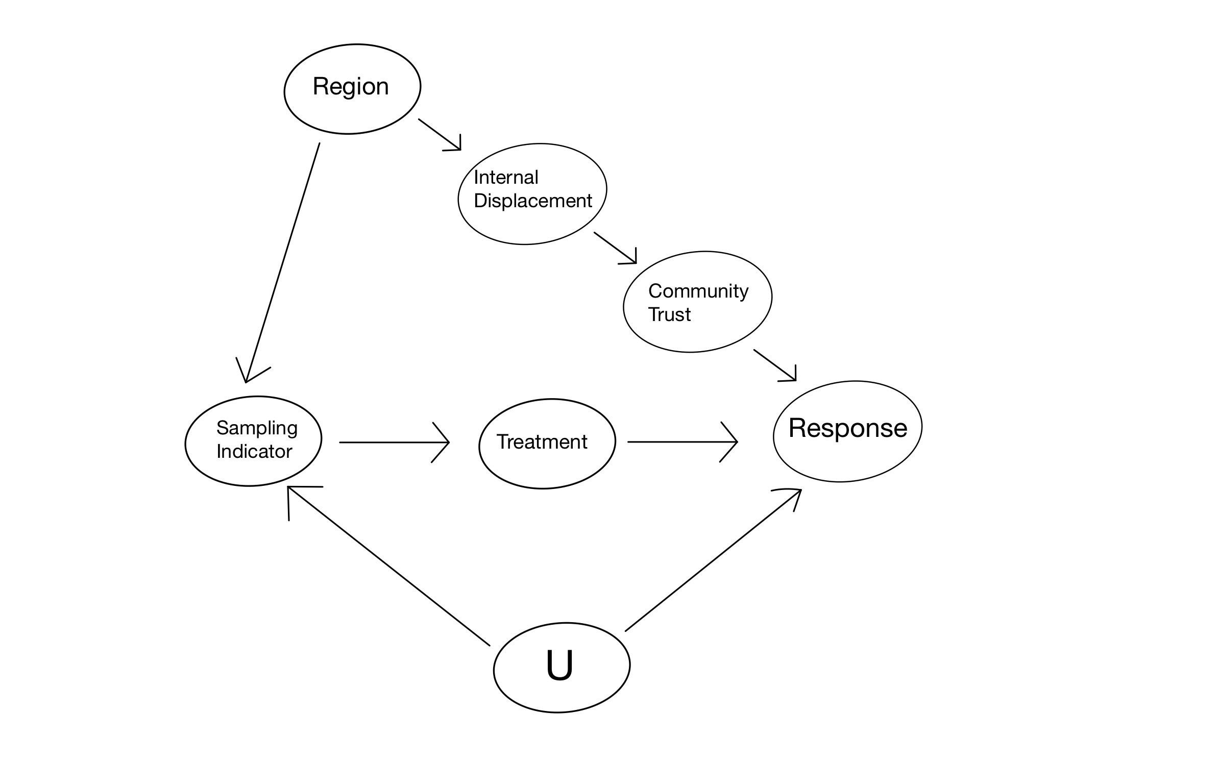
If \(U\) acts as an effect modifier and is unobserved, then we no longer have the identification of our population average treatment effect. Neither Community Trust nor Internal Displacement are valid adjustment sets any longer. Are we out of luck? Not completely. While we won’t be able to pin down our PATE entirely, we can do the following: First, we suspend our belief momentarily, pretend that \(U\) doesn’t exist, and estimate the PATE as we did before when \(U\) wasn’t around. Then, we can attempt to understand how the existence of \(U\) drives bias in the estimate we have produced. In particular, we try to understand what \(U\) would have to be like in order to bias our estimate so drastically that it overturns our putative results. If \(U\) being like this seems implausible, then our results are safe. This procedure is known as sensitivity analysis.
Procedure
When we used {Community Trust} as our adjustment set to estimate the PATE in the last blog post, our estimator was
\[ \widehat{PATE_C} = \sum_c\widehat{SATE_c}P_{\Omega_t}(C=c), \] where \(C\) is community trust.
This estimator can actually be re-written in Horvitz-Thompson form:
\[ \widehat{PATE_C} = \frac{1}{n_1}\sum_{i\in\Omega_s}w_iT_iY_i - \frac{1}{n_0}\sum_{i\in\Omega_S}w_i(1-T_i)Y_i, \] where the weights are given by \(w_i = \frac{P(S_i=1)P(S_i=0 \mid C_i)}{P(S_i=0)P(S_i=1 \mid C_i)}\).
Melody Huang develops a framework for sensitivity analysis for PATE estimators of this form here. There, she shows the following result:
Assume \(Y(1) - Y(0) \perp\!\!\!\perp S \mid \{C, U\}\). Let \(w_i\) be the weights estimated using only \(C_i\), i.e.
\(w_i = \frac{P(S_i=1)P(S_i=0 \mid C_i)}{P(S_i=0)P(S_i=1 \mid C_i)}\) and let \(w_i^*\) be the correct weights estimated using \(\{C_i, U_i\}\), i.e. \(w_i^* = \frac{P(S_i=1)P(S_i=0 \mid C_i, U_i)}{P(S_i=0)P(S_i=1 \mid C_i, U_i)}\). Then the bias of the estimator \(\widehat{PATE_C}\) is given by
\[ Bias(\widehat{PATE_C}) = \begin{cases}\rho_{\varepsilon, \tau} \sqrt{\operatorname{var}_{\Omega_s}\left(w_i\right) \cdot \frac{R_{\varepsilon}^2}{1-R_{\varepsilon}^2} \cdot \sigma_\tau^2} & \text { if } R_{\varepsilon}^2<1 \\ \rho_{\varepsilon, \tau} \sqrt{\operatorname{var}_{\Omega_s}\left(w_i^*\right) \cdot \sigma_\tau^2} & \text { if } R_{\varepsilon}^2=1\end{cases} \]
This formula requires some explaining. First, define \(\tau_i = Y_i(1)-Y_i(0)\) to be the individual treatment effects and \(\varepsilon_i=w_i - w_i^*\) to be the differences between the weights we estimate for adjusting with only Community Trust and the true weights for adjusting with Community Trust and U. Now, the three parameters appearing in the formula are defined as follows:
\(\rho_{\varepsilon, \tau}\) is the correlation between the weight residuals \(\varepsilon_i\) and the treatment effects \(\tau_i\) among the units in the experiment
\(\sigma_\tau^2\) is the variance of the treatment effects among the units in the experiment
\(R_\varepsilon^2\) is the ratio of the variance of \(\varepsilon_i\) and the variance of \(w_i^*\) among the units in the experiment
In addition to this result, Huang shows the following two lemmas:
The variance of the true weights decomposes as
\[ \operatorname{var}_{\Omega_s}(w_i^*) = \operatorname{var}_{\Omega_s}(w_i) + \operatorname{var}_{\Omega_s}(\varepsilon_i) \]
Therefore, \(R_\varepsilon^2 := \frac{\operatorname{var}_{\Omega_s}(\varepsilon_i)}{\operatorname{var}_{\Omega_s}(w_i^*)}\) is bound between 0 and 1.
The correlation between \(\varepsilon_i\) and the individual-level treatment effects \(\tau_i\) is bound in the following way:
\[ -\sqrt{1-\operatorname{cor}_{\Omega_S}(w_i, \tau_i)} \leq \rho_{\varepsilon, \tau} \leq \sqrt{1-\operatorname{cor}_{\Omega_S}(w_i, \tau_i)} \]
These results in tandem provides a path forward for performing sensitivity analysis for generalizing experimental results:
- Estimate an upper bound for \(\sigma_\tau^2\), i.e. \(\sigma_{\tau,max}\). Huang provides some suggestions on this front, but the upper bound that I find most obvious, if not most efficient, comes from assuming that the potential outcomes under treatment are positively correlated with the potential outcomes under control. We then have
and variances of the potential outcomes can be estimated unbiasedly from the observed data thanks to randomization.
- Using \(\sigma_{\tau,max}\), estimate a lower bound for \(\operatorname{cor}_{\Omega_S}(w_i, \tau_i)\), i.e. \(\operatorname{cor}^{min}_{\Omega_s}(w_i, \tau_i)\). This can be done straightforwardly since
- Using \(\operatorname{cor}^{min}_{\Omega_S}(w_i, \tau_i)\), form the upper bound on \(|\rho_{\varepsilon, \tau}|\) given in Lemma 3.3: \[ |\rho_{\varepsilon, \tau}| \leq \sqrt{1-\operatorname{cor}^{min}_{\Omega_s}(w_i, \tau_i)}\]
- Vary \(R_\varepsilon^2\) from 0 to 1 and \(\rho_{\varepsilon, \tau}\) from \(-\sqrt{1-\operatorname{cor}_{\Omega_s}^{min}(w_i, \tau_i)}\) to \(\sqrt{1-\operatorname{cor}_{\Omega_s}^{min}(w_i, \tau_i)}\) and for each pair of values, use the formula in Theorem 3.1 to calculate the bias in the estimate of the PATE:
\[ Bias(\widehat{PATE_C}) \lessapprox \rho_{\varepsilon, \tau} \sqrt{\operatorname{var}_{\Omega_s}\left(w_i\right) \cdot \frac{R_{\varepsilon}^2}{1-R_{\varepsilon}^2} \cdot \sigma_{\tau,max}^2}, \]
the symbol \(\lessapprox\) suggesting that, because we’re using \(\sigma_{\tau,max}^2\) instead of \(\sigma_{\tau}^2\), we should in theory have an upper bound on the bias.
We can then check whether any such \(|\rho_{\varepsilon, \tau}|\) and \(R_\varepsilon^2\) generate a bias larger in absolute value than the estimate itself, i.e. \(|Bias(\widehat{PATE_C})| > |\widehat{PATE_C}|\), which would constitute the overturning of our putative result i.e. the sign of our estimator would be wrong.